


To learn more, explore all available Courses.
Your DCF valuation is only as credible as your discount rate, yet many analysts still plug in outdated risk premiums while the 10-year Treasury yield sits at a hawkish 5.00%. You understand that the capital asset pricing model is the definitive industry standard for determining the cost of equity. However, applying it in a volatile 2026 market requires more than just a basic textbook formula. It demands the professional judgment of an industry insider who knows how to pivot when equity risk premiums are compressed to historic lows.
This guide will move you beyond academic theory to master the mechanics of the capital asset pricing model, ensuring you can build institutional-grade models that stand up to rigorous committee scrutiny. We’ll break down the precise steps to source the risk-free rate, correctly lever and unlever beta, and implement these calculations directly into Excel. You’ll gain the confidence to defend every assumption in high-stakes interviews or investment meetings. This is the blueprint for performing at the level of elite industry practitioners.
To learn more, explore all available Courses.
To learn more, explore all available Courses.
The capital asset pricing model serves as the primary mechanism for determining the required rate of return on equity. It’s not just a theoretical exercise. In the high-stakes world of investment banking and private equity, it’s the foundational tool that bridges the gap between risk and valuation. By quantifying the relationship between systematic risk and expected return, analysts can establish a hurdle rate that reflects the true cost of equity for any firm. This precision is vital for capital allocation decisions.
At its core, the model relies on three critical inputs: the Risk-Free Rate (Rf), Beta (β), and the Equity Risk Premium (ERP). With the 10-year U.S. Treasury yield reaching 5.00% in September 2026, the baseline for risk-free assets has shifted, forcing professionals to re-evaluate their discount rates. The model integrates these variables to provide a clear, defensible output that feeds into the Weighted Average Cost of Capital (WACC). It’s the industry’s most trusted method for aligning asset pricing with Modern Portfolio Theory.
Modern finance dictates that investors shouldn’t be compensated for risk they can easily eliminate through diversification. This is why the capital asset pricing model focuses exclusively on systematic risk, also known as non-diversifiable risk. While idiosyncratic risks are specific to a single company, systematic risks are inherent to the entire market. Understanding the Capital Asset Pricing Model requires a firm grasp of the Security Market Line (SML). The SML provides a visual representation of this trade-off, plotting expected returns against Beta to show how much additional yield an investor requires for every unit of market risk they assume.
Despite the emergence of multi-factor models, CAPM remains the dominant choice for calculating the cost of equity in 2026. Its staying power stems from a perfect balance of simplicity and institutional acceptance. While models like Fama-French offer more complexity, they often introduce too much noise for standard deal-making. Professional analysts use CAPM as the standard baseline for DCF valuation because it provides a transparent and universally understood framework. It’s the language of the industry. Mastering this model is the first step toward building models that command respect in any committee meeting.
To learn more, explore all available Courses.
To learn more, explore all available Courses.
The capital asset pricing model formula is deceptively simple: Re = Rf + β(Rm – Rf). In this equation, Re represents the expected return on equity, which functions as the foundational cost of equity for your valuation model. While the calculation is straightforward, your professional credibility hinges on the precision of your inputs. Analysts must maintain strict consistency across time horizons. If you’re projecting cash flows over a ten year period, your risk-free rate and equity risk premium must reflect that same duration. Using a short term T-bill yield against a long term market premium creates a fundamental mismatch that can invalidate your entire WACC. Despite its ubiquity, empirical tests of the CAPM highlight that the model isn’t infallible, particularly when beta fails to capture the full spectrum of market risk.
In the high yield environment of September 2026, the 10-year U.S. Treasury yield has reached 5.00%, serving as the professional benchmark for the risk-free rate. It’s the standard because it lacks default risk and matches the duration of most institutional investment horizons. When you’re modeling for international markets, you can’t simply swap in a local government bond rate if that nation carries sovereign risk. In those cases, professionals subtract the country’s default spread from the local bond yield to isolate the true risk-free component. The current hawkish monetary policy means your Rf is no longer a static “set and forget” input; it’s a dynamic variable that reflects 2026’s persistent inflationary trends.
The ERP represents the excess return investors demand over the risk-free rate to compensate for market volatility. It’s the “Rm – Rf” portion of the formula. As of March 2026, implied equity risk premiums have been estimated between 4.25% and 4.55%, sitting near historic lows. This presents a critical judgment call. You must decide whether to use forward looking implied rates, which reflect current market pricing, or historical averages that might be higher but account for long term cycles. In volatile sectors, analysts often lean toward conservative estimates to ensure their models aren’t overly optimistic. If you’re ready to apply these judgment calls to institutional-grade models, our DCF Valuation Course provides the professional framework you need.
To learn more, explore all available Courses.
To learn more, explore all available Courses.
Beta measures how much an asset’s price fluctuates compared to the broader market index. It is the core metric for systematic risk. While platforms like Bloomberg or Yahoo Finance provide raw regression Betas, professional analysts rarely use them at face value. These figures are often backward-looking and heavily skewed by a company’s specific capital structure during the look-back period. If the market has shifted or the company has recently changed its debt profile, these raw numbers are obsolete. To achieve precision, you must derive a Beta that reflects the business risk of your target company independently of its financing. Beta is the only component of risk that the capital asset pricing model rewards.
To isolate pure business risk, analysts use a process called unlevering. This removes the financial distortion caused by debt. You start by identifying a set of comparable peers and gathering their levered Betas. Using the standard unlevering formula, or the Hamada Equation, you strip out the impact of each peer’s specific debt-to-equity ratio and marginal tax rate. This results in an Asset Beta, which represents the risk of the operations alone. Once you calculate an industry average Asset Beta, you must re-lever it using your target company’s projected capital structure. This technical workflow is a staple in private equity modeling, where the goal is often to transform a company’s leverage profile significantly. Mastering this conversion ensures your cost of equity reflects the future state of the business, not its historical debt levels.
Precision in the capital asset pricing model depends on the quality of your peer group. You aren’t looking for clones, but for companies with similar operating leverage and revenue drivers. Select companies that mirror your target in terms of industry focus, revenue size, and geographic exposure. A group of at least 5-10 peers is generally required to ensure the average is statistically significant and less prone to individual company noise. Watch for outliers. If one peer has a Beta of 2.5 while the rest of the set sits near 1.1, investigate the cause immediately. It might be due to extreme financial distress or a recent idiosyncratic shock. If the outlier doesn’t reflect the industry norm, exclude it to preserve the integrity of your average. Your final Beta must be a defensible reflection of the systematic risk inherent in the sector.
To learn more, explore all available Courses.
To learn more, explore all available Courses.
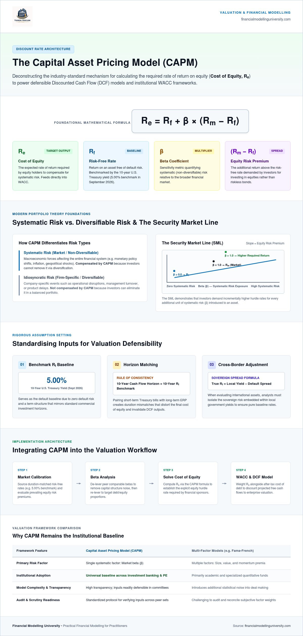
The output of the capital asset pricing model is the engine that drives your entire valuation. It provides the Cost of Equity (Re), which is the most subjective and impactful component of the Weighted Average Cost of Capital (WACC). Unlike the Cost of Debt, which is observable through market yields or bank spreads, the Cost of Equity must be estimated. It’s almost always higher than the cost of debt because equity holders sit at the bottom of the capital stack. They take on the residual risk of the business. If the company fails, debt holders are paid first; equity holders are paid last. This increased risk profile demands a higher return premium, which CAPM quantifies for your model.
Terminal value often represents over 70% of a DCF’s total value. Since the discount rate is used to capitalize the terminal year cash flow, even a 50-basis-point error in your CAPM calculation can lead to massive valuation distortions. Precision here is not optional. Professional analysts always perform sanity checks by comparing their implied WACC against industry averages. If your discount rate is a significant outlier compared to peers, you must have a technical justification ready for your investment committee.
In a standard DCF, WACC functions as the discount rate for free cash flows. The formula integrates your CAPM-derived Re with the after-tax cost of debt, weighted by their respective market values. Small shifts in your Beta or Equity Risk Premium (ERP) can swing a company’s Enterprise Value by millions of dollars. For example, a 0.10 increase in Beta in a high-growth model can significantly compress the present value of future cash flows. To handle these complex calculations without error, follow the spreadsheet best practices outlined in our Excel for Finance guide.
Professional analysts never rely on a single point estimate for valuation. Instead, they build sensitivity tables in Excel to test how the capital asset pricing model inputs affect the final price. By varying Beta and the ERP across a defined range, you can identify a valuation range that accounts for market volatility. This is where you separate yourself from juniors. When an investment committee or interviewer asks why you chose a specific Beta, you must be prepared to defend your range. Mastering these institutional-grade workflows is essential for career advancement. Enroll in our DCF Valuation Course to start building models like the pros.
To learn more, explore all available Courses.
To learn more, explore all available Courses.
Mastering the capital asset pricing model is a prerequisite for any serious finance professional. However, knowing the formula isn’t the same as defending a valuation in a high-pressure environment. FMU bridges the gap between academic theory and the practical precision required by elite firms. We don’t just teach you how to calculate numbers; we show you how to interpret them like an industry insider. This shift in perspective is what separates a standard analyst from a professional who commands respect. You need to understand the logic behind every input to survive an investment committee’s scrutiny.
Junior analysts often struggle to transition from textbook exercises to live deal modeling. FMU courses solve this by using real-world case studies that mirror actual investment banking workflows. You’ll get hands-on experience with the same tools used at the top of the industry. This includes access to downloadable CAPM templates and sophisticated peer comp sheets that automate the levering and unlevering process. These resources ensure your models are structured correctly from day one, reducing the risk of technical errors. One-to-one mentoring is also available to help you navigate the most complex valuation hurdles. This personalized guidance provides a level of clarity that automated tutorials simply can’t match.
In the competitive 2026 job market, prestige matters. Holding an FMU certification signals to employers that you’ve mastered the rigorous standards of corporate finance. More than 25,000 finance professionals have already trusted FMU to accelerate their careers. Top-tier banks and private equity firms look for candidates who can hit the ground running without extensive hand-holding. By mastering the capital asset pricing model and DCF models through Financial Modelling University, you position yourself as a high-value asset. Whether you choose the DCF Valuation Course or the FMU All-Access Pass, you’re investing in your own career trajectory. You’ll gain the technical confidence to navigate the most challenging technical interviews with ease. It’s time to stop learning and start performing at an elite level.
To learn more, explore all available Courses.
To learn more, explore all available Courses.
Professional valuation is an exercise in precision and defensibility. You’ve learned how to deconstruct the capital asset pricing model to isolate systematic risk and apply hawkish 2026 market rates to your DCF models. By refining your beta calculations and aligning your risk premiums with current economic realities, you move beyond academic theory into institutional-grade practice. This level of technical mastery is what separates elite practitioners from the rest of the field.
FMU is trusted by 25,000+ finance professionals who seek career transformation through industry-recognized certifications. Our curriculum provides the blueprint for success, offering elite mentorship from former investment banking pros who have operated at the highest levels of the industry. Take the next step in your professional journey and master financial modeling like the pros today. You have the tools to build models that command respect in any committee meeting.
To learn more, explore all available Courses.
To learn more, explore all available Courses.
The capital asset pricing model is a financial framework that calculates the expected return on an investment based on its systematic risk. It functions as a precise bridge between the risk-free rate and the additional premium investors demand for holding volatile assets. Professionals use it to determine the cost of equity, ensuring that every institutional valuation model accounts for the inherent trade off between non-diversifiable market risk and potential reward.
You calculate the cost of equity by adding the risk-free rate to the product of the stock’s Beta and the equity risk premium. The formula is Re = Rf + β(Rm – Rf). For a professional result in 2026, you must use a risk-free rate of 5.00% and a defensible Beta derived from comparable peers. This calculation provides the essential discount rate for your DCF valuation, reflecting the minimum return equity holders expect for their capital.
Beta is the only component of risk that the capital asset pricing model rewards. It measures the sensitivity of an asset’s returns relative to the broader market. A Beta of 1.0 indicates the asset moves in lockstep with the market, while a Beta above 1.0 suggests higher volatility. In professional modeling, Beta captures the non-diversifiable, systematic risk that can’t be eliminated through a broad portfolio, making it the primary driver of the equity premium.
In 2026, a professional equity risk premium (ERP) typically ranges between 4.25% and 4.55% based on March 2026 estimates. This forward looking figure reflects the compressed premiums seen in current market conditions. While historical averages might suggest a higher ERP, using these specific 2026 figures ensures your model remains grounded in actual institutional expectations. Analysts must exercise judgment when selecting an ERP, especially when evaluating sectors with unique risk profiles or during periods of low market volatility.
Yes, CAPM is the standard for private company valuation, though it requires an indirect approach. Since private firms lack a public stock price, you must source Betas from a group of comparable public peers. Analysts unlever these peer Betas to isolate business risk and then re-lever the average based on the private company’s specific capital structure. This workflow allows professionals to apply the capital asset pricing model with institutional precision to non-public entities without guessing the cost of equity.
The model’s main limitations include its reliance on historical data to predict future returns and its assumption of perfect market efficiency. It only accounts for systematic risk, ignoring idiosyncratic factors that might impact a specific firm. Critics also point out that the single factor Beta often fails to capture the full complexity of modern market dynamics. Despite these theoretical flaws, its simplicity and transparency make it the most widely accepted tool for calculating the cost of equity in investment banking.
Investment banks like JP Morgan and Goldman Sachs continue to use CAPM as the foundational method for calculating the cost of equity in DCF models. It remains the industry standard because it provides a clear, defensible framework that all market participants understand. While elite analysts might use multi factor models for niche research, CAPM is the primary language used during investment committee meetings and high level negotiations to justify discount rate assumptions and final enterprise values.
The risk-free rate serves as the foundational floor for all expected returns in the formula. As the risk-free rate increases, the overall cost of equity rises, which in turn lowers the present value of future cash flows in a DCF model. With the 10-year U.S. Treasury yield reaching 5.00% in September 2026, hurdle rates have shifted significantly higher. This trend makes government bonds more attractive relative to equities and forces a more conservative valuation environment for analysts.
To learn more, explore all available Courses.