


A cost of equity calculation isn’t a static formula; it’s a defensive argument for a company’s risk profile. In the high-stakes environment of investment banking, a single misstep in your ke assumptions can invalidate an entire DCF valuation. Most junior analysts falter when choosing between levered and unlevered Beta or sourcing reliable 2026 Equity Risk Premium data. You know the frustration of staring at a terminal, wondering if your CAPM inputs will survive a senior committee’s scrutiny.
At FMU, we understand that professional mastery requires more than academic theory. This guide promises to transform your technical approach, providing the blueprint to calculate ke with institutional-grade accuracy. You’ll learn to navigate the complexities of private company valuations and implement these formulas efficiently in Excel. We’ll break down the mechanics of the Capital Asset Pricing Model, the nuances of industry-specific risk adjustments, and the exact steps to defend your valuation assumptions like an elite practitioner. Master financial modeling like the pros and ensure your next model stands up to the highest industry standards.
The cost of equity (ke) represents the minimum rate of return a company must offer to satisfy its shareholders for the specific risk of their investment. It’s the price of ownership. In elite finance, we view ke as a strategic hurdle rate. If an internal project or a potential acquisition doesn’t exceed this rate, you’re essentially destroying shareholder value. A precise cost of equity calculation ensures that capital is only deployed where it generates a surplus above the investors’ required return.
In the 2026 market, this calculation has become more critical than ever. Risk-free rates have stabilized at higher levels than the previous decade. This shift elevates the baseline for all equity investments, making capital more expensive and narrowing the margin for error in valuation models. Professionals can’t rely on outdated assumptions; they must understand how these macro shifts impact the bottom line.
Opportunity cost is the value of the next best alternative foregone when a specific capital allocation decision is made.
Debt and equity sit at opposite ends of the risk spectrum. Debt is senior; lenders get paid first, which lowers their risk and, consequently, the Cost of Debt (kd). Equity holders are the residual claimants. They take on the most risk and demand a significantly higher premium. A professional cost of equity calculation must reflect this inherent risk hierarchy to be considered institutional-grade.
The tax-shield advantage also separates the two. Interest on debt is tax-deductible, reducing the effective kd. Equity offers no such benefit. As we navigate 2026, many firms are re-evaluating their capital structures. With the higher cost of debt, equity premiums are being squeezed. This forces analysts to be more rigorous in their ke assumptions. Mastering these nuances is a core component of the DCF Valuation Course at FMU, where we bridge the gap between academic theory and real-world execution.
The Capital Asset Pricing Model (CAPM) remains the industry standard for any rigorous cost of equity calculation. It distills complex market risks into a linear equation that elite analysts use to defend their valuation floors. The formula is straightforward: ke = Rf + β × (Rm – Rf). While the math is simple, the precision of your model depends entirely on the quality of your inputs. In 2026, the “higher-for-longer” interest rate environment means your Risk-Free Rate (Rf) shouldn’t be a historical average; it must reflect current 10-year or 20-year Treasury yields to capture the true baseline cost of capital.
The Equity Risk Premium (ERP), or (Rm – Rf), represents the excess return investors demand over risk-free assets. In a post-inflationary 2026 economy, this premium is sensitive to shifting growth expectations. Professionals rely on forward-looking ERP data rather than just historical means to ensure their models reflect current market sentiment. If your inputs are stale, your entire valuation is compromised.
Beta measures a security’s volatility relative to the market. Analysts often face a choice between Raw Beta and Adjusted Beta. Bloomberg typically uses the 0.33/0.67 rule to adjust Raw Beta toward the market mean of 1.0, assuming that over time, idiosyncratic risks revert to the average. When valuing private companies or divisions, you’ll need to “unlever” the Betas of comparable public peers to remove the effect of debt, then “relever” that average based on your target’s specific capital structure. Use this checklist for selecting peer groups:
The ERP is the most debated input in a cost of equity calculation. While historical data provides a long-term anchor, elite practitioners prioritize the implied ERP data published by experts like Aswath Damodaran. This forward-looking approach accounts for current earnings yields and dividend growth. For valuations involving international entities, you must add a Country Risk Premium (CRP) to the base US ERP. This adjustment accounts for political instability, currency volatility, and sovereign default risk. Mastering these technical adjustments is exactly what we cover in the DCF Valuation Course, ensuring your models are built on institutional-grade foundations rather than guesswork.
Elite valuation isn’t about one formula; it’s about defensibility. Relying solely on CAPM can leave your model vulnerable during a rigorous M&A audit. Professional practitioners often use alternative models to cross-check their cost of equity calculation, ensuring the final figure reflects the asset’s true risk profile. Triangulating between different methodologies allows you to present a range of values, which is the standard for institutional-grade reports.
While CAPM accounts for systematic market risk, it can sometimes miss the nuances of specific company types or sectors. By implementing multiple frameworks, you build a “valuation bridge” that supports your final assumptions. This disciplined approach is what separates a junior analyst from a master of the craft.
For mature, stable entities with predictable payout histories, the Gordon Growth Model (GGM) offers a market-implied alternative. The formula is: ke = (D1 / P0) + g. In this equation, D1 represents the next year’s expected dividend, P0 is the current stock price, and g is the constant growth rate. You can estimate ‘g’ with precision by multiplying the firm’s retention ratio by its Return on Equity (ROE). This method is highly effective for utilities or consumer staples. However, it’s virtually useless for high-growth tech firms that reinvest 100% of their earnings. In those scenarios, CAPM remains the more reliable tool.
When you’re valuing private companies where comparable public Betas are scarce or unreliable, the Build-Up Method is the professional’s choice. Instead of relying on market volatility, you stack specific risk premiums. This method is a staple in private equity and lower middle-market M&A. The structure typically follows this progression:
Defending your “Alpha” adjustment is the hardest part of a valuation committee review. You must justify this specific risk based on tangible factors like customer concentration, management depth, or key-man dependencies. Mastering these qualitative adjustments is a core pillar of the DCF Valuation Course. Analysts who can articulate the “why” behind their cost of equity calculation components move to the front of the pack in private equity interviews. They don’t just provide a number; they provide a narrative backed by technical rigor.
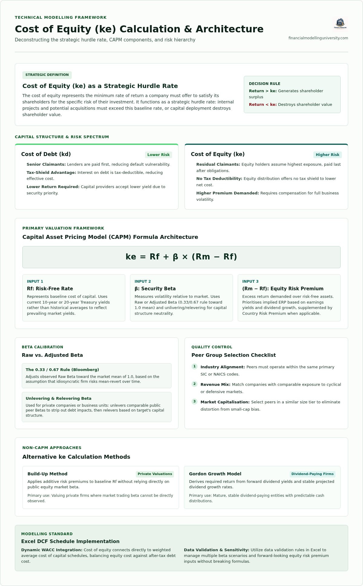
A professional DCF is only as good as its underlying architecture. You shouldn’t bury your cost of equity calculation in a hidden cell on the valuation tab. Instead, build a dedicated “WACC Schedule” within your multi-sheet model. This ensures transparency and allows senior reviewers to audit your assumptions instantly. Use Excel for Finance best practices to maintain clean, logical flows. Implement data validation with drop-down menus to toggle between different Beta sources or ERP scenarios, making your model dynamic and robust. This structural discipline reflects the precision required at the elite levels of investment banking.
Start by listing your peer group in a structured table. Include columns for ticker, name, market cap, total debt, cash, and the marginal tax rate. Calculate the Debt/Equity (D/E) ratio for each. To find the asset risk, you must unlever the observed market Betas. Use the formula: βu = βl / [1 + ((1 – t) * (D/E))]. Once you have the unlevered Betas, calculate the peer median to mitigate the impact of outliers. Relever this median Beta using your target company’s capital structure. Avoid hard-coding any values; use dynamic cell references so that updating a single tax rate or debt figure ripples through the entire model. This prevents manual errors and ensures your cost of equity calculation remains institutional-grade.
Valuation is never a single point; it’s a range. Set up a 2-variable Data Table to sensitize Enterprise Value against changes in ke and the Terminal Growth Rate. This table provides the data points needed for a “Football Field” chart, which visually compares your DCF results against M&A multiples and LBO returns. In Excel, navigate to Data, What-If Analysis, Data Table to link your discount rate and growth inputs. For professional presentation, format the “implied” cost of equity cells with custom borders or conditional formatting to highlight the base case. This level of granularity allows you to defend your valuation floor during intense committee questioning.
Mastering these technical workflows is essential for anyone aiming for the bulge bracket. You can perfect your modeling speed and accuracy by enrolling in our Excel for Finance Course today.
In an investment banking interview, your ability to execute a flawless cost of equity calculation is the ultimate technical litmus test. It’s not just about the math; it’s about your capacity to justify every input under intense pressure. Senior bankers look for candidates who understand how macro shifts in 2026 influence the discount rate. A Financial Modeling Certification serves as a powerful signal to the industry. It validates that you’ve moved beyond surface-level tutorials to achieve a professional standard of excellence recognized by global firms.
Success in elite finance requires more than just knowing a formula. You must understand how ke interacts with the broader capital structure to drive investment decisions. This is the core philosophy of our Investment Banking Financial Modeling Course. We’ve trained over 25,000 finance professionals using institutional-grade methods that bridge the gap between academic theory and high-stakes execution. By mastering these technicalities, you position yourself as a strategic architect rather than a mere spreadsheet operator.
Elite analysts don’t just calculate numbers; they build narratives. They explain why a specific size premium was chosen or why a peer group was narrowed down to three specific companies. This narrative ability is what separates the top 1% of candidates. Through our one-to-one career mentoring, you’ll learn to articulate your assumptions with the confidence of a seasoned associate. Our case studies use real-world data, forcing you to navigate the same ambiguities and technical hurdles faced by practitioners at bulge-bracket banks. You’ll gain the instinctual understanding of risk that only comes from disciplined, expert-led practice.
Professional mastery is a structured progression. Once you’ve perfected the cost of equity calculation, the next step is integrating it into complex transaction structures like LBO Modeling. This is where you see the real-world impact of your WACC assumptions on internal rates of return (IRR) and equity multiples. To accelerate this journey, the FMU All-Access Pass provides the comprehensive training needed to dominate the recruitment cycle and perform on day one.
Don’t leave your career to chance. Download our professional DCF template today to begin practicing these institutional-grade techniques immediately. Master Financial Modeling Like the Pros with FMU University and transform your professional trajectory with the blueprint used by industry leaders.
A rigorous cost of equity calculation is the foundation of any institutional-grade valuation. You’ve learned to navigate the nuances of the CAPM framework, implement alternative models like the Build-Up method, and build dynamic, auditable WACC schedules in Excel. These aren’t just technical exercises; they’re the tools used by elite analysts to defend multi-billion dollar assumptions. Mastery of these skills transforms you from a spreadsheet operator into a strategic architect.
Don’t leave your professional development to chance. Master Institutional-Grade Valuation in our DCF Course and gain access to the same downloadable Excel templates used by over 25,000 pros. With mentorship from elite finance pros and an industry-recognized certification, you’ll be prepared to lead the high-stakes conversations that define the top tier of the industry. Take the next step toward professional prestige today.
Calculate ke for a private entity by using the Build-Up Method or a peer-group comparable analysis. Since private firms lack a traded share price, you must unlever the Betas of public peers to isolate business risk, then relever the median Beta using the private company’s specific target debt-to-equity ratio. Add a size premium and a company-specific risk premium to account for the lack of liquidity and smaller operational scale.
A “good” rate is entirely dependent on the specific risk profile of the asset, but 2026 market expectations for mature US equities typically range between 8% and 12%. This reflects a stabilized 10-year Treasury yield near 4% and a standard equity risk premium. High-growth technology sectors or distressed industries will naturally command significantly higher rates to compensate investors for increased volatility and idiosyncratic risk.
You must use levered beta in the final CAPM formula. Levered beta accounts for both the inherent business risk and the financial risk created by the company’s capital structure. Unlevered beta is only used as an intermediate step to normalize risk across a group of comparable companies. Once you find the peer median unlevered beta, you must relever it to match your target’s leverage before finishing the cost of equity calculation.
Inflation drives the cost of equity higher by increasing the nominal risk-free rate. When central banks maintain higher interest rates to manage price levels, the baseline return required by all investors rises. Furthermore, persistent inflation can expand the equity risk premium if it creates uncertainty around future corporate earnings. This dual pressure makes equity capital more expensive, forcing a more disciplined approach to project selection and valuation floors.
Cost of equity (ke) is the required return specifically for shareholders, while WACC is the blended cost of all capital sources, including debt and preferred equity. Because equity holders are the last to be paid in a liquidation, ke is virtually always higher than the cost of debt. WACC serves as the discount rate for the entire firm, whereas ke is the specific rate used when discounting cash flows available only to equity holders.
The 10-year Treasury yield is the industry standard because its duration aligns with the long-term investment horizon of a typical DCF model. It’s the most liquid and widely accepted proxy for a default-free asset. Using a shorter-term instrument, like a 3-month T-bill, would fail to capture the long-term opportunity cost of capital and would introduce unnecessary volatility into your cost of equity calculation.
Source the ERP from institutional-grade providers like Kroll or the implied ERP data published by Aswath Damodaran. Professional analysts in 2026 prioritize forward-looking implied premiums over historical averages. This approach calculates the premium based on current market prices and expected future cash flows, ensuring your model reflects today’s economic reality rather than the average performance of the last several decades.
No, the cost of equity cannot be negative. Investors demand a positive return to compensate for the risk of losing their principal and the uncertainty of future dividends. Even in a low-interest-rate environment, the equity risk premium remains positive because equity is a residual claim. A negative ke would imply that shareholders are willing to pay the company for the privilege of owning its risky stock, which contradicts fundamental economic logic.