Build a Simple LBO Model: Debt Paydown and Exit Returns

A leveraged buyout model succeeds or fails on the discipline of its debt schedule. When you set out to build LBO model architecture in Excel, small errors in your cash sweep or circular interest formulas can quickly distort your entire return profile. You likely know the frustration of watching a sources and uses table refuse to balance, or wrestling with spreadsheet errors while trying to prioritise senior and mezzanine tranches under tight deadlines.

A reliable model eliminates that guesswork by anchoring capital structure mechanics in clear, disciplined cash flow logic. In this tutorial, you will learn how to construct a fully integrated leveraged buyout model from a blank worksheet. We will cover establishing entry assumptions, building an error-free debt paydown waterfall without fragile circular references, and forecasting dynamic MoIC and IRR exit returns with total confidence.

Establish Transaction Assumptions and the Sources and Uses Schedule

Every transaction evaluation begins with clean purchase price mechanics. When you set out to build LBO model architecture, opening balance sheet adjustments and ongoing cash sweeps depend directly on an accurate Sources and Uses schedule. An unverified assumption here corrupts every downstream returns forecast.

Calculating Purchase Price and Capital Structure Inputs

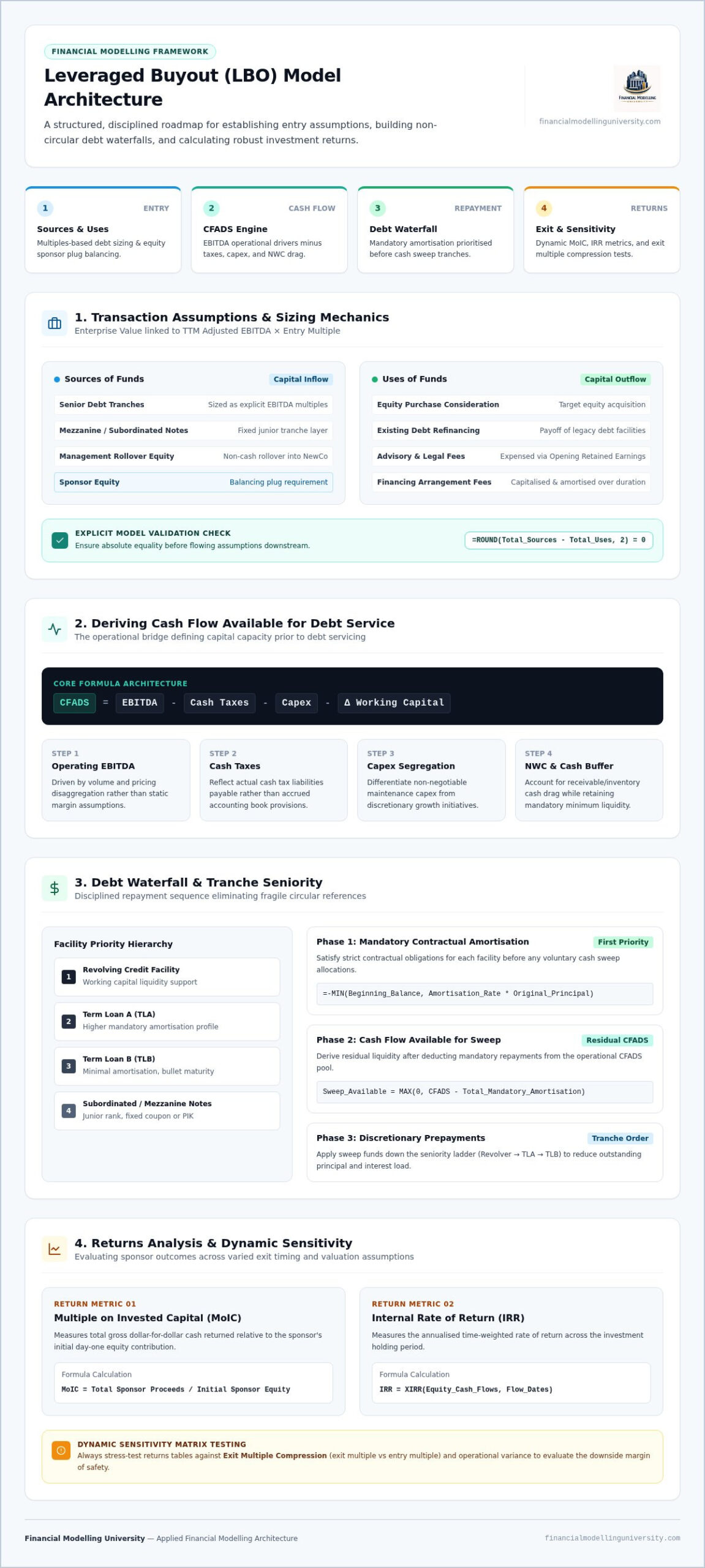
First, link enterprise value to trailing twelve-month (TTM) adjusted EBITDA and an entry valuation multiple. To understand the foundational mechanics of a Leveraged Buyout (LBO), remember that debt sizing depends on debt-to-EBITDA limits rather than enterprise value percentages. Set senior debt and subordinated debt tranches as explicit multiples of EBITDA. Sponsor equity acts as the balancing plug, combined with any management rollover equity that rolls into the new holding company without cash leaving the deal.

Constructing the Sources and Uses Table

A robust Sources and Uses schedule categorises capital properly and reconciles transaction costs on the opening balance sheet:

• Sources: Group new senior debt, mezzanine notes, sponsor funds, and rollover equity.
• Uses: Allocate cash toward the equity purchase, existing debt payoff, and distinct fee pools.
• Fee Accounting: Differentiate advisory fees, which expense immediately through opening retained earnings, from financing fees, which capitalise on the balance sheet and amortise over the loan duration.

Always insert an explicit validation check cell: =ROUND(Total_Sources - Total_Uses, 2) = 0. Ensuring this equation holds true lets you build LBO model structures that balance seamlessly from day one.

Forecast Operating Performance and Cash Available for Debt Service

Operating projections dictate your ultimate debt capacity. While simplified templates often treat cash generation as a fixed percentage margin, you need granular operational drivers to build LBO model forecasts that hold up under technical scrutiny.

Projecting Operating Drivers and EBITDA Margins

Start by separating revenue into volume and pricing components across distinct business units. Project cost of sales and operating expenses against these volume drivers rather than assuming static EBITDA margins. As detailed in Harvard’s leveraged buyout model overview, establishing realistic operational baselines forms the core of transaction assessment. Anchor depreciation schedules to existing fixed-asset registers and planned asset additions.

Deriving Free Cash Flow Available for Debt Service

Cash Flow Available for Debt Service (CFADS) defines the operational cash pool available to service interest, scheduled amortisation, and prepayments. Unlevered cash flow excludes financing impacts entirely, whereas CFADS serves as the direct operational feeding mechanism for the debt schedule before interest deductions occur.

• Adjust EBITDA: Deduct cash taxes payable rather than accrued accounting provisions.
• Subtract Capital Expenditures: Distinguish non-negotiable maintenance capex from growth initiatives.
• Factor Working Capital: Account for the cash drag created by growing receivables and stock requirements.
• Enforce Minimum Cash: Retain a mandatory liquidity buffer so the company covers day-to-day working capital needs.

The core formula resolves to: CFADS = EBITDA - Cash Taxes - Capex - Change in NWC. This dynamic pool directly drives your debt waterfall without distorting solvency. To practise implementing these operating bridges across complex transaction scenarios, explore our applied financial modelling courses.

Build the Debt Schedule with Waterfall and Circularity Breakers

The debt schedule governs capital structure prioritisation and cash distribution. When you build LBO model workbooks, establishing a strict hierarchy between mandatory amortisation and voluntary prepayments ensures debt pays down without breaching loan agreements.

Layering Debt Tranches and Repayment Waterfalls

Structure debt facilities by seniority: revolving credit facility, Term Loan A, Term Loan B, and subordinated notes. Apply cash against obligations using this precise waterfall:

• Mandatory Amortisation: Satisfy contractual principal repayments first using formula logic: =-MIN(Beginning_Balance, Amortisation_Rate * Original_Principal).
• Cash Flow Available for Sweep: Calculate remaining cash after subtracting mandatory repayments from operational CFADS.
• Discretionary Prepayments: Sweep excess cash into senior facilities before subordinate tranches: =-MIN(Beginning_Balance + Mandatory_Repayment, Remaining_Sweep_Cash).
• Commitment Fees: Apply the fee percentage exclusively against the undrawn revolver balance.

Managing Circular References and Interest Calculations

Calculating interest expense on average debt balances creates an immediate circular reference. Ending cash depends on net income, net income depends on interest expense, and interest expense depends on ending debt balances. In Excel, this circular loop can cause #NUM! or #REF! calculation crashes if iterative calculations stall.

Break this loop by installing a dedicated circularity toggle cell (for instance, cell C5 set to 1 for ON, 0 for OFF). Structure your interest formula as follows:

=IF($C$5=1, AVERAGE(Beginning_Balance, Ending_Balance), Beginning_Balance) * Interest_Rate

Setting the switch to 0 bases interest solely on beginning balances, allowing you to build LBO model logic and debug cash flows safely. Once cash flows balance, toggle the switch to 1. To practise building automated waterfalls and circularity toggles with downloadable templates, explore our applied financial modelling courses.

Calculate Returns Metrics and Conduct Dynamic Sensitivity Analysis

Returns metrics reveal whether a transaction generates sufficient compensation for financial risk. When you build LBO model returns modules, link final payouts directly to closing debt balances rather than relying on static estimates.

Deriving Exit Equity Value, MoIC, and IRR

Begin by defining an investment horizon, typically five years. Calculate exit enterprise value by applying a terminal multiple to final-year EBITDA: Exit_EV = Final_EBITDA * Exit_Multiple. Subtract ending net debt to derive exit equity value distributed to shareholders.

• Multiple on Invested Capital (MoIC): Divide total ending cash returned to the financial sponsor by initial sponsor equity invested: =Exit_Equity / Entry_Equity.
• Internal Rate of Return (IRR): Apply the XIRR function against exact transaction dates to capture cash flow timing accurately.
• Value Creation Drivers: Deconstruct total returns into operational EBITDA growth, debt paydown, and multiple expansion to identify what actually creates investment value.

Stress-Testing Models via Dynamic Data Tables

An acquisition thesis must withstand multiple contraction. Build standard two-way data tables using Excel Data Tables (Alt + A + W + T) to test IRR and MoIC across different exit multiples and leverage levels.

Excel data tables calculate every combination dynamically. If your workbook recalculates slowly or crashes, set calculation options to “Automatic Except for Data Tables” under Excel settings. This isolates table processing until manual calculation (F9) occurs. For a step-by-step walkthrough of these valuation techniques and returns waterfalls, review practical advanced frameworks in our LBO Financial Models online course.

Take Command of Your Transaction Modelling Workflow

Constructing reliable transaction spreadsheets requires strict mechanical discipline. When you build lbo model templates from a blank worksheet, every component must align seamlessly, from balancing the Sources and Uses table to isolating debt repayment waterfalls with dependable circularity breakers. Stress-testing these mechanics against multiple compression ensures your returns analysis reflects genuine credit risk and operational reality rather than optimistic assumptions.

Putting these principles into practice sharpens your ability to evaluate acquisitions quickly and defend your figures under scrutiny. To reinforce your technical skills with structured guidance, explore the practical financial modelling courses at Financial Modelling University. You’ll gain access to downloadable Excel models and templates alongside hands-on financial modelling exercises designed around actual transaction workflows. Open a blank workbook today and turn complex leverage mechanics into an instinctive modelling habit.

Frequently Asked Questions

What is the difference between an LBO model and a standard DCF model?

A DCF model evaluates intrinsic enterprise value by discounting unlevered free cash flows at a weighted average cost of capital. In contrast, you build LBO model logic to determine the equity returns (IRR and MoIC) generated by a target company under an explicit debt structure and exit timeline. While a DCF solves for business valuation, an LBO evaluates whether a specific transaction price delivers acceptable financial returns to the sponsor.

How do you calculate Cash Flow Available for Debt Service in an LBO?

Calculate Cash Flow Available for Debt Service (CFADS) by deducting cash taxes, net working capital increases, and capital expenditures directly from adjusted EBITDA. This metric establishes the actual operational cash pool remaining to service debt obligations before deducting interest expenses or principal payments. It ensures your repayment schedule models real operational cash generation rather than abstract accounting profits, preventing unfeasible debt paydown forecasts.

Why do LBO models frequently create circular reference warnings in Excel?

Circular references occur when interest expense is calculated using the average of beginning and ending debt balances. Ending debt depends on the discretionary cash sweep; the cash sweep depends on net cash generation; net cash generation depends on net interest expense; and interest expense relies on ending debt. Without a binary toggle switch to break this loop during audits, Excel enters a continuous calculation cycle that can trigger calculation errors.

What is an acceptable sponsor IRR and MoIC target in leveraged buyouts?

Private equity sponsors typically target a gross Internal Rate of Return (IRR) between 20% and 25%, alongside a Multiple on Invested Capital (MoIC) between 2.0x and 2.5x over a standard five-year holding period. In higher interest rate environments with lower available leverage, sponsors rely less on multiple expansion and prioritise operational improvements and margin expansion to satisfy these hurdle rates for institutional fund investors.

Can you build a simple paper LBO model without complex Excel schedules?

Yes, analysts frequently build paper LBO models during early transaction screening or private equity interviews. Instead of dynamic schedules, you use round numbers, approximate cumulative cash conversion as a percentage of EBITDA, and apply simplified mandatory debt repayments. This streamlined approach lets you build LBO model returns estimates in under ten minutes, demonstrating whether an acquisition warrants detailed three-statement modelling and deeper due diligence.