


A single historical beta isn’t the only defensible input for a DCF. A practical Damodaran beta alternative is a bottom-up estimate: use comparable companies to assess each business’s operating risk, then adjust for the company’s business mix and debt. This approach can be more useful when a firm’s own share-price history is short or its operations span different sectors.
Beta measures sensitivity to market movements, not a company’s total risk. Diversification can reduce business-specific risk, while the company’s business mix and leverage shape the equity beta used in valuation. For a diversified company, the estimate should reflect its operations, not only how its shares have moved.
This article explains how diversification affects equity beta and compares bottom-up estimates with regression, accounting-based and factor-based approaches. It also covers how factor models capture market risk through several return drivers and when each method is useful in a financial model. The goal is a beta assumption you can explain, test and link to the cost of equity.
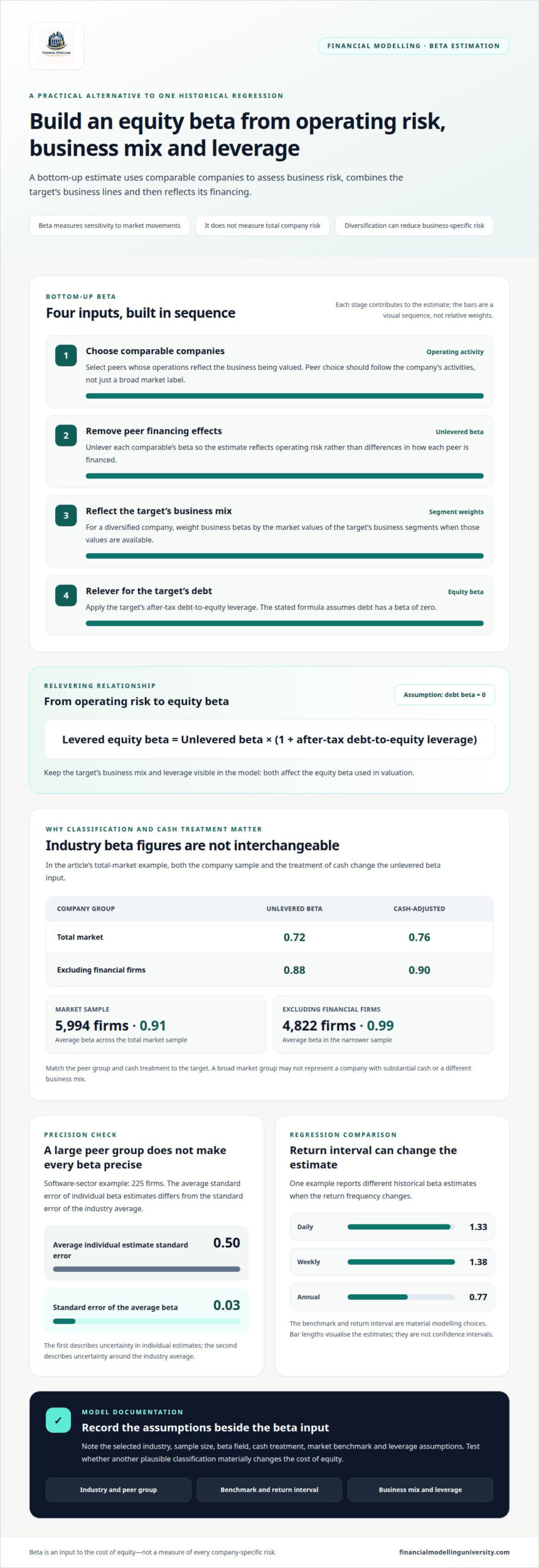
Equity beta measures a stock’s sensitivity to market returns, while diversification changes how much company-specific risk remains. The total market sample averages 0.91 across 5,994 firms; excluding financial firms, it averages 0.99 across 4,822 firms.
Raw beta is the slope from regressing a company’s historical returns against market returns; adjusted beta moves that estimate towards the market average. Adjustment can temper an unusually high or low historical estimate, but it may also obscure a genuine change in the company’s risk. For example, Disney’s S&P 500 beta estimate is 1.13, with a standard error of 0.22 and a 95% confidence interval of 0.69 to 1.57.
Providers can report different betas for the same company because their benchmarks, return frequencies and estimation windows may differ. Beta equals correlation with the market multiplied by the stock’s standard deviation divided by the market’s standard deviation. Compare those inputs before choosing a figure: an S&P 500 beta and a global-index beta measure exposure to different markets.
Historical regression estimates beta as the covariance of stock and market returns divided by market-return variance. Use matching observations and dates; monthly returns can provide sufficient observations for firms listed for more than three years. Estimates can shift with frequency: an example reports 1.33 using daily returns, 1.38 using weekly returns and 0.77 using annual returns. These differences make the benchmark and return interval material modelling choices.
A bottom-up estimate starts with comparable firms’ unlevered betas, then accounts for the target’s business mix and leverage. Select peers by operating activity, remove the effect of their financing, and weight the business betas by the market values of the target’s business segments when available. Assuming debt has zero beta, levered equity beta equals unlevered beta multiplied by one plus after-tax debt-to-equity leverage. This approach is useful for companies with several business lines or limited trading history.
Beta captures market-related risk, not every company-specific risk, so CAPM cost of equity can miss risks that diversification may reduce. In a DCF, document the beta, market benchmark and leverage assumptions alongside the other cost-of-equity inputs; the DCF and valuation modelling context helps connect those assumptions to the valuation.
Damodaran’s industry tables are most useful when you treat each beta field as a distinct modelling input, rather than interchangeable headline figures. First match the table’s company group to the target, then select the measure that reflects the target’s financing and cash position. The column you choose should follow from the valuation logic.
For example, the total market has an unlevered beta of 0.72 and an unlevered beta corrected for cash of 0.76. Without financial firms, those figures are 0.88 and 0.90. The difference shows why sample composition and cash treatment matter. A target with substantial cash may be poorly represented by a measure that leaves cash unadjusted; a target with a different business mix may not fit the overall-market group.
Read industry sample size and estimate precision together. In a software-sector example covering 225 firms, the average beta-estimate standard error was 0.50, while the standard error of the average beta was 0.03. The first describes uncertainty in individual estimates; the second describes uncertainty around the industry average. A large peer group can make an average more stable without making every constituent beta precise.
In an Excel valuation, note the selected industry, sample size, beta field and cash treatment beside the input. Then test whether another plausible classification materially changes the cost of equity. This sensitivity shows whether the valuation relies on a robust industry signal or a narrow grouping choice. Use Damodaran’s tables as structured evidence, and make the reason for each selected figure clear to reviewers.
A regression beta is not the only way to assess risk. In the page’s example, the beta estimated from quarterly returns was 0.44. Telebras’s relative volatility against the average Brazilian stock was estimated at 0.80, using annualized standard deviations of 48% and 60%. These measures capture different aspects of risk, so the choice should fit the valuation question and available data.
A bottom-up beta estimates the betas of a firm’s businesses using average regression betas of publicly traded firms in each business, then adjusts for differences in financial leverage. It uses business-specific unlevered betas, weighted by the market values of the firm’s businesses when those values are available. Accounting data offer another route: quarterly accounting statements over five years provide 20 observations for an accounting beta regression.
A Damodaran beta alternative should suit the company’s operations and the risk your valuation needs to capture. Compare peer-industry estimates, factor-based measures and market indices, then document why the chosen reference fits the business. Don’t select a method simply because it produces a preferred valuation.
Industry and peer references help when a company’s activities differ from a broad market average. The available industry estimates show why classification matters: semiconductor firms average a beta of 1.52, while general utilities average 0.24. Software (Internet) averages 1.69, compared with 1.21 for advertising. These figures are useful reference points, not automatic inputs. Check whether the company’s revenue drivers resemble the firms grouped in its proposed industry.
Factor-based approaches provide a different comparison by measuring exposure to multiple return drivers rather than relying on one industry-wide figure. Meketa presents annual returns of alternative-beta indices for 2005 through 2014. For valuation work, use a factor approach when the company’s risk profile isn’t captured well by a single market relationship. Keep the factor definition and risk-premium assumptions visible so reviewers can see what the estimate represents.
Low-volatility indices can serve as a reference for businesses with defensive characteristics. Meketa estimated a market beta of 0.76 for the S&P 500 Low Volatility Index over April 1995 to March 2015. Its analysis describes low volatility as an observed anomaly, with low-volatility or low-beta portfolios outperforming higher-volatility portfolios over long periods. Treat that historical result as context, not as a forecast for an individual company.
Other risk measures can provide a useful cross-check when market-price evidence is weak. Accounting-based and option-implied approaches draw on different evidence from industry beta tables, so compare what each measure captures before using it in the cost of equity. For analysts translating these risk parameters into ongoing mandate oversight, Market Ontology provides portfolio risk tools and investment research that extend beyond static beta tables. A sound choice makes the valuation assumption easier to explain, challenge and update as the company’s business mix changes.
The semiconductor industry’s unlevered beta is 1.49; its cash-corrected unlevered beta is 1.50. Software (Internet)’s cash-corrected unlevered beta is 1.59. Regional banking’s 568-firm sample averages 0.40; its unlevered beta is 0.29 and cash-corrected unlevered beta is 0.37.
Bloomberg, Capital IQ and Refinitiv provide beta estimates, but the figure alone doesn’t reveal which settings produced it. The standard calculation relates a stock’s returns to a market benchmark using correlation and relative return volatility. Differences in benchmark, return frequency or estimation window can therefore produce different estimates for the same company.
Begin by recording the benchmark beside each figure. An estimate against the S&P 500 represents exposure to that index, while one against a global index captures a different market relationship. Next, note whether the input uses daily, weekly or monthly returns. The chosen frequency changes which price movements enter the estimate and how observations align.
Next, compare the estimation windows. A shorter period may give more weight to recent trading conditions, while a longer one covers more historical market environments. Neither is automatically better. Choose a period that suits the valuation purpose and apply it consistently across the companies being compared. Also check whether the figure is raw or adjusted, since an adjustment changes the historical estimate.
For a reproducible Excel check, align stock and index returns by date, then calculate the regression slope. In SLOPE, enter stock returns as known y-values and index returns as known x-values. Check date alignment and return intervals before comparing your result with Bloomberg, Capital IQ or Refinitiv. Differences in these inputs can explain a gap without indicating a calculation error.
Keep a concise audit note of the provider, benchmark, frequency, observation window and adjustment status. If estimates still differ, compare the underlying return series and settings before choosing an input. This turns a platform figure into a traceable assumption that reviewers can reproduce and challenge in the valuation model.
Financial Modelling University offers practical training for analysts who want to build valuation assumptions into working Excel models. The LBO Financial Models online course covers building an LBO model, where financing assumptions flow into debt schedules and investor returns. For DCF valuation, the DCF & Valuation online course is a closer fit, covering how cost-of-equity inputs connect to cash-flow valuation.
Both courses include step-by-step video lessons, downloadable Excel models and templates, and practical financial modelling exercises. Use these materials to practise documenting beta assumptions and tracing their effects through a model, rather than treating the estimate as an isolated input. Choose the course that fits the model you’re building.
Visit financialmodellinguniversity.com to explore the course options.
Carry the selected beta into your model as a documented assumption, not a hard-coded figure without context. Record its source, benchmark, return frequency, estimation period and adjustment status. For a bottom-up estimate, retain the peer set, business weights and leverage adjustment so another reviewer can trace the calculation.
Then test how changes in beta affect the cost of equity and DCF value. Keep the sensitivity linked to the model’s formulas, and explain whether a valuation difference comes from the beta method or another assumption. A Damodaran beta alternative is appropriate when its logic fits the company and valuation purpose, not simply because it produces a preferred result.
Use the same discipline in future models: make assumptions visible, keep calculations consistent and leave a clear audit trail. Explore financial modelling courses to develop your modelling practice. Keep refining the logic behind each input, and you’ll build valuations you can explain with confidence.