Top LBO Model Pitfalls to Avoid for Clean Financials

A clean-looking LBO model can still misstate returns when operating forecasts and the debt schedule do not connect. Common LBO modelling pitfalls include unsupported revenue or margin assumptions, overlooked working capital needs, and mixing operating cash flow with financing flows.

An LBO model projects a business’s performance after an acquisition funded partly with debt. It links operating drivers to cash available for interest and debt repayment, then shows how remaining debt and exit value affect investor returns. The challenge is keeping every link transparent and consistent.

This article explains how to build and test revenue, cost and cash flow drivers, separate operating cash from financing movements, and assess the trade-offs of traditional LBO modelling. It also shows why exit timing and exit multiple can materially change projected returns, and how model checks can expose errors before they distort your conclusion.

Separating financing cash flows from operating cash flow

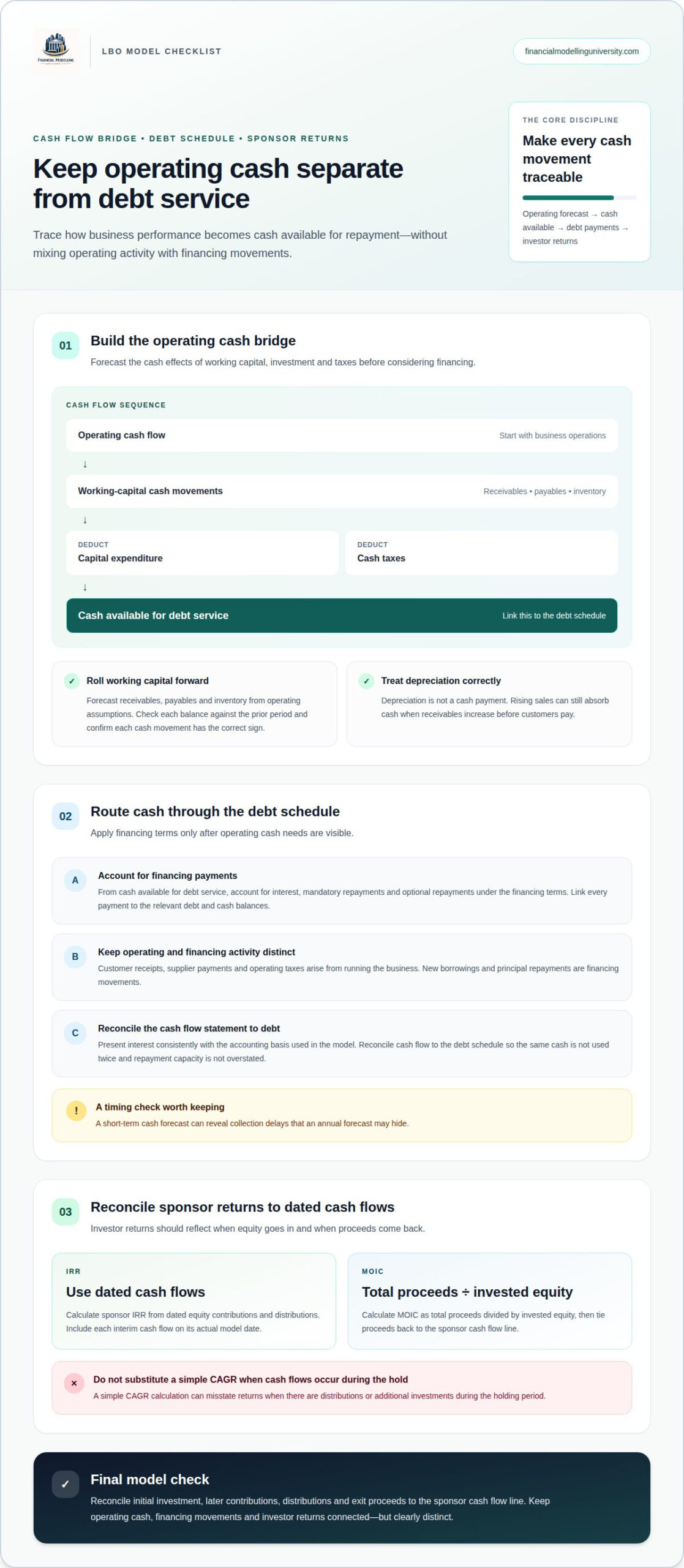
Build the cash flow bridge to keep operating performance, investment needs and financing movements distinct. This makes cash available for debt service traceable to the forecast, rather than an assumption based on EBITDA alone.

1. Forecast Working Capital, Capital Expenditures, and Taxes

   Forecast receivables, payables and inventory from operating assumptions, then calculate changes in those balances as cash movements. For example, rising sales may increase receivables when customers pay after revenue is recognised. Subtract capital expenditure and cash taxes in the operating cash flow bridge, but do not treat depreciation as a cash payment. Check that working capital balances roll forward from the prior period and that each cash movement has the correct sign.

2. Link Free Cash Flow to Debt Repayments

   Calculate cash available for debt service from operating cash flow after working capital, capital expenditure and cash taxes. Then account for interest, mandatory repayments and optional repayments under the financing terms. Link each payment to the relevant debt and cash balances. This prevents the model from using the same cash twice or showing repayment capacity the operating forecast does not generate.

3. Keep operating and financing activity separate in the cash flow statement. Customer receipts, supplier payments and operating taxes arise from running the business; new borrowings and principal repayments are financing movements. Present interest consistently with the accounting basis used in the model, then reconcile the cash flow statement to the debt schedule. A short-term cash forecast can also reveal collection delays that an annual forecast may hide.
4. Calculate sponsor IRR from dated equity contributions and distributions, and MOIC as total proceeds divided by invested equity. A common mistake is using a simple CAGR calculation when distributions or additional investments occur during the holding period. Include each interim cash flow on its actual model date, and reconcile the initial investment, later contributions, distributions and exit proceeds to the sponsor cash flow line.

What are the advantages and disadvantages of traditional LBO modelling?

A traditional LBO model connects acquisition assumptions to projected sponsor returns in a structured framework. Its strength is transparency; its limitation is that outputs can look precise even when key assumptions remain uncertain.

1. Calculate entry enterprise value by multiplying the target’s reference EBITDA by the selected entry multiple. Then bridge enterprise value to the purchase price and funding requirement, accounting for cash, debt and transaction uses. This separates valuation from funding and clarifies which assumptions drive the sponsor equity required at acquisition.
2. Build a sensitivity table for exit multiple and exit timing. Show how each combination changes exit enterprise value, equity proceeds, IRR and MOIC. The table makes return exposure easier to assess, but may still imply more certainty than the assumptions justify. Label the base case and explain what each alternative represents.
3. Base the exit multiple on evidence, then test lower and higher outcomes. Avoid carrying the entry multiple forward automatically without considering the target’s projected performance and market position at exit. If the investment case relies on multiple expansion, show it separately from EBITDA growth and debt reduction. This distinguishes operational value creation from valuation change.
4. Extend scenario analysis beyond valuation. Build a downside case that changes relevant operating assumptions and exit timing together, then review liquidity, debt capacity and projected returns. Traditional models provide a disciplined way to compare cases, but isolated sensitivities may miss interacting pressures. Keep each scenario internally consistent so it represents a coherent investment outcome.
5. Place model checks beside the outputs. Confirm acquisition sources equal uses, debt balances roll forward correctly, and the balance sheet balances in every forecast period. Reconcile enterprise value to equity value through net debt, and ensure sponsor proceeds tie to the exit calculation. These checks can catch formula errors, but they cannot establish whether an investment assumption is commercially sound.

Debt financing sources and typical terms

Debt structure affects cash available for repayment and the equity remaining at exit. Model each financing source from its documented terms, not a generic assumption.

1. Set Debt Structure and Financing Terms

   Enter each tranche separately, using its contractual principal, interest rate, maturity, fees and repayment priority. Link interest expense to the relevant balance and rate, and reflect rate changes only when the financing terms support them. Reconcile total debt sources to the transaction’s funding requirements alongside sponsor equity. Avoid blending tranches, which can hide differences in cost, maturity and claim priority.

2. Schedule Mandatory and Optional Repayments

   Build mandatory repayment rules from the loan terms, then calculate optional repayments from cash remaining after operating needs and required payments. Roll each tranche forward as opening balance plus borrowing, less principal repayments. Apply optional repayment in the specified order and stop when the relevant balance is repaid. This avoids reducing debt twice or allocating cash the target needs to operate.

3. Assess Debt Coverage and Leverage

   Calculate leverage as debt divided by the EBITDA measure used in the financing analysis. Calculate debt service coverage by comparing cash available for debt service with scheduled principal and interest, using consistent periods and definitions. Review both measures under lower-earnings and higher-interest scenarios. A single base case can obscure liquidity pressure, so track cash balances alongside coverage and repayment capacity.

4. Test how financing terms affect leveraged buyout returns. Higher interest expense reduces cash available for repayment, while slower amortisation can leave more debt outstanding at exit. Compare closing debt with the balance produced by each period’s borrowing and repayment calculations. Include fees in the appropriate transaction uses or financing cash flows, and check that debt balances reconcile across the schedule and balance sheet.

Model drivers and income statement projections

1. Start with operating evidence, not a growth rate chosen to support the purchase price. In a worked example, £20.0 million of revenue and £4.0 million of adjusted EBITDA imply a 20% EBITDA margin. Build revenue from measurable inputs, such as units produced, prices, customer volumes or retention, then link each assumption to the relevant forecast line. A common LBO modelling mistake is forecasting growth without showing its operating basis.
2. Translate capacity into revenue where production drives sales. One illustrative case models eight factories producing four million widgets initially, or 500,000 widgets per factory. Forecast output by facility, then apply the assumed selling price. This structure makes a capacity constraint visible; a simple growth percentage can otherwise imply sales the business cannot deliver. Compare projected output with available production capacity in every forecast period.
3. Project margins through specific costs, not an unexplained EBITDA uplift. An example case increases EBITDA margin from 20% to 25%; show which operating costs or productivity changes support that movement. Test the assumptions separately, since higher volume may not improve margins if labour, materials or other costs rise alongside revenue. Another common LBO modelling mistake is assuming margin expansion without identifying its drivers.
4. Complete the income statement and link it to cash flow. An illustrative model assumes annual depreciation and amortisation of $5 million, capital expenditure equal to 10% of sales each year, and a 35% tax rate per year. Calculate EBIT as EBITDA less depreciation and amortisation, then apply the tax assumption consistently. Keep capital expenditure separate from depreciation because it affects cash flow directly.
5. Run a coherent downside and compare its effect on valuation and returns. Traditional LBO models often project performance over 5-7 years; test slower growth or margin pressure across that horizon, rather than changing one input in isolation. Reconcile revenue, EBITDA, taxes and cash generation before assessing debt paydown and exit value. A sound analysis makes each assumption traceable from operating performance through to investor returns.

Financial Modelling University: Project Finance Modeling Course Now Available

Financial Modelling University’s LBO Financial Models online course is a practical next step for learning to build and check the debt schedule, operating forecast and sponsor returns in an integrated Excel model. Course materials include downloadable Excel models and templates, along with practical financial modelling exercises. Use this structured practice to test how changes in revenue, working capital, interest and repayments flow through to returns, and to strengthen your model review process. For valuation work that complements LBO analysis, the DCF & Valuation online course covers a related modelling area. Contact Financial Modelling University to discuss which course fits your learning goals.

Make the next model easier to audit

The lbo model pitfalls to avoid are easier to control when every assumption is traceable in the spreadsheet. Carry that discipline into your next model: label inputs, separate calculations from hard-coded values, and connect operating forecasts, financing movements and sponsor returns with clear formulas. Then test whether changes in operating drivers flow through to cash, debt and equity value without breaking the model checks.

Use the finished model as a decision tool, not just a return calculator. A clear structure helps colleagues challenge assumptions, compare scenarios and understand what drives the investment case. If you want to practise building and reviewing financial models, explore Financial Modelling University’s courses and choose a learning path that fits your next modelling goal.

Keep strengthening the links between assumptions and outputs. Consistent checks and a transparent structure can help you approach your next LBO model with greater confidence.

Frequently Asked Questions

What is an LBO model?

An LBO model is an Excel forecast used to analyse an acquisition financed with debt and investor equity. It connects the target’s operating performance and financing to the sponsor’s potential proceeds at exit. For example, it can show how a change in sales volume affects EBITDA, cash available for debt repayment and the equity value remaining when the business is sold.

What are the three drivers of returns in an LBO?

The three core drivers are EBITDA growth, debt reduction and the change in the enterprise value multiple between entry and exit. EBITDA growth can increase exit value if the exit multiple holds, while debt repayment can increase the equity share of that value. Multiple expansion can also raise proceeds, but it adds valuation risk rather than improving operations.

What is the right exit multiple assumption?

No single exit multiple suits every transaction. Set a base case using the target’s expected position at exit, its earnings profile and relevant valuation evidence. Then test a range around that case. If returns depend on an exit multiple higher than the entry multiple, make that reliance clear and examine whether operating progress supports the difference.

What are the most common LBO modelling mistakes?

Common errors include hard-coded outputs, inconsistent signs, broken links between schedules and formulas that double-count cash flows. For example, a repayment may reduce debt on the balance sheet without reducing cash in the cash flow schedule. Trace key outputs back to their inputs, test formulas across forecast periods and confirm the model balances after changing assumptions.

What are common mistakes when forecasting revenue, margins, and operating cash flow?

A frequent forecasting mistake is applying one growth rate to every revenue stream, even when volumes, prices or customer mix change differently. Margin forecasts may also assume scale benefits without linking them to specific costs. For cash flow, align receivables, payables and inventory with the operating forecast; otherwise, projected profit may not convert to cash on schedule.

How do you calculate management fees, transaction fees, and other deal expenses?

Model each expense using its agreed basis and timing instead of combining costs in one plug. Calculate a management fee using its stated rate and defined base, and build transaction expenses from relevant deal cost assumptions. Record each item once, in the correct period and schedule. At closing, include applicable transaction expenses in uses so funding sources reconcile to total uses.