NPV vs XNPV in Excel: A Worked Cash-Flow Timing Example

A project can appear to destroy value in one spreadsheet and create value in another, even when both contain the same cash amounts. Before changing the discount rate, check the dates. A formula that treats an early receipt as a payment several years away can distort the answer enough to reverse its sign.

The practical difference between NPV and XNPV in Excel is the clock each function uses. NPV discounts by equally spaced periods; XNPV discounts by specified payment dates. For cash flows tied to actual dates, that distinction deserves as much attention as the amounts themselves.

This guide builds one hypothetical example, checks the result independently and shows how a 90-day collection delay changes value. All amounts are USD. The assumed 12% annual effective discount rate is an illustration, not a recommended rate or a market estimate.

NPV vs XNPV: the difference that matters

Microsoft describes NPV as a periodic calculation: each entry falls at the end of the next equal period. Its rate must match that period. An annual model needs an annual rate; a monthly model needs a monthly rate. A cash payment made immediately belongs outside the NPV function, added separately.

XNPV takes a rate, cash amounts and corresponding dates. Excel uses the first date as its valuation anchor and discounts using elapsed days divided by 365. Include the initial investment alongside later receipts in the dated range. These are different timing conventions, so the functions need not agree even when supplied with identical amounts.

Choose the convention before building the formula. If your forecast assumes one payment at each year-end, periodic NPV can represent that assumption. If a contract specifies staged payments, use those dates rather than assigning every receipt to a convenient annual column.

Worked example: the same receipts, different timing

Suppose a business pays $100,000 on 1 January 2026 for a project. It expects three net cash receipts: $30,000 after 90 days, $40,000 after 365 days and $50,000 after 730 days. Treat these as complete project cash flows for this teaching example; no additional tax, financing, terminal-value or working-capital items are implied.

The undiscounted receipts total $120,000, giving a $20,000 surplus over the initial payment. Discounting reduces that surplus because future dollars carry less present value at the assumed positive rate. Here, the discounted receipts total $104,747.26, leaving a positive NPV of $4,747.26.

That is a result under the stated cash amounts, timing and rate. It does not establish that the project should be approved: an omitted payment, an unrealistic collection date or a mismatched risk assumption could change the conclusion.

Build the XNPV formula in Excel

Use a compact input area that makes the assumptions visible. Enter 12% in B1. Put the heading “Date” in A3 and “Cash flow” in B3. Enter the four dates in A4:A7 and the corresponding amounts in B4:B7, starting with −100000 in B4.

Use real Excel dates. For an unambiguous first entry, type =DATE(2026,1,1) in A4. The remaining dates are =DATE(2026,4,1), =DATE(2027,1,1) and =DATE(2028,1,1). Displaying a cell as a date is useful, but the underlying value must also be a date rather than a text label.

Calculate the dated project value with:

=XNPV($B$1,B4:B7,A4:A7)

The result is $4,747.26, measured at 1 January 2026. Do not subtract B4 again: the negative initial investment is already in the range. Preserve full precision in formulas and round only the displayed outputs.

Build a transparent second calculation alongside it. In C4, enter =A4-$A$4 and copy down to C7. In D4, enter the formula below and copy it down to D7:

=B4/(1+$B$1)^(C4/365)

Sum D4:D7. This row-by-row calculation should match XNPV. It also makes review easier: the initial outflow stays undiscounted, while the three later receipts use exponents of 90/365, 1 and 2. In a larger model, those visible exponents help reveal dates that were accidentally linked to the wrong forecast column.

Why a periodic NPV can give the opposite answer

Now use the same cash amounts with an annual periodic formula:

=NPV($B$1,B5:B7)+B4

This returns −$5,737.52. The function has not malfunctioned. Its inputs now describe receipts one, two and three annual periods from the investment date. That differs from the intended schedule of 90, 365 and 730 days.

The gap is $10,484.78. It comes from a changed timing assumption, not a change in the cash amounts. Calling the periodic answer “more conservative” would hide the actual issue: it is valuing a different schedule. Either schedule could be appropriate if it matches the project being modelled, but they cannot both describe these supplied payment dates.

For an immediate investment plus three genuine annual receipts, the periodic formula above would be appropriate. Placing the initial investment inside NPV($B$1,B4:B7) would introduce another mistake by discounting that immediate payment for one period.

Stress-test a 90-day delay

Keep the investment date and all cash amounts fixed, then delay every positive receipt by 90 days. In F4, enter =A4. In F5, enter =A5+90 and copy down to F7. Calculate:

=XNPV($B$1,B4:B7,F4:F7)

The delayed result is $1,860.72. Compared with the original case, value falls by $2,886.55, or approximately 60.8% of the original net present value. This percentage concerns the small surplus after the investment; it is not a 60.8% fall in gross receipts or total discounted inflows. Receipts still total $120,000.

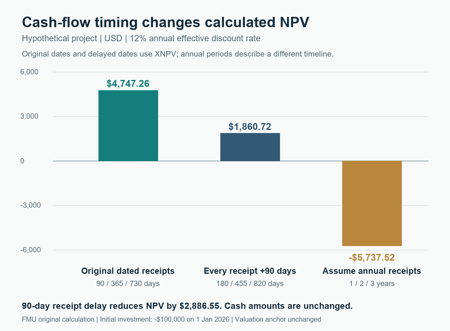
Original FMU calculation. The third bar assumes different receipt dates and illustrates a modelling mismatch; it is not another forecast scenario for the supplied schedule.

View the chart at full size.

This is a useful sensitivity because it isolates collection timing. A fuller downside case might also reduce receipts, add costs or change the rate, but combining every change at once makes the source of the valuation movement harder to explain. Start with one driver, establish the mechanism, then build a combined case with explicit assumptions.

Choose a rate that matches your timing convention

The example assumes a 12% annual effective rate throughout. If you build a monthly periodic model using that same effective annual assumption, the equivalent monthly rate is:

=(1+12%)^(1/12)-1

That produces approximately 0.948879% per month. Compounding it for 12 months returns 12%. Simply dividing 12% by 12 gives 1% per month, which compounds to approximately 12.6825% annually. A nominal annual rate quoted with monthly compounding is a different input convention and should be documented accordingly.

Calendar months also have unequal day counts. Converting a rate does not make monthly period-end discounting identical to XNPV’s dated calculation. Decide whether the model needs a periodic approximation or precise scheduled dates, and label that choice.

Rate selection itself requires a separate justification. Keep currency, inflation treatment and the cash-flow definition consistent with the rate you choose. If that assumption is under review, FMU’s guide to the DCF assumptions that matter provides broader forecasting context.

Checks before sharing the model

Review the timeline independently of the formulas. Ask whether the date represents invoice issuance, contractual payment or expected cash collection. If the model is meant to value cash receipts, linking to an invoice date can introduce an optimistic assumption even when every formula is correct.

Then check these five items:

1. Valuation anchor: Is the first date the date at which you intend to measure value?
2. Range alignment: Does every amount have exactly one corresponding date?
3. Sign convention: Is the investment negative and each receipt positive from the same party’s perspective?
4. Completeness: Have you captured all relevant cash items once, including any final payment?
5. Independent reconciliation: Does the manual discounted sum agree with the main result within a rounding tolerance?

Keep the original and delayed dates side by side. Overwriting the base dates makes the sensitivity difficult to audit and can leave a reviewer unable to reproduce the earlier answer. Record the scenario name, timing change and output together. For a wider review process, use FMU’s financial-model audit guide.

Frequently asked questions

Is XNPV always better than NPV?

Use the function that matches the intended timeline. A periodic forecast can reasonably use NPV when equal spacing is an explicit assumption. Known irregular payment dates call for a dated calculation. XNPV cannot repair incorrect or incomplete cash-flow inputs.

Why can two dated models still disagree?

Compare the valuation anchor, rate, amounts and dates before comparing headline outputs. One model may value the project at investment close while another uses a later reporting date. Also check whether a final receipt or investment has been included twice.

Does a positive result mean the project is attractive?

It means the modelled receipts exceed the investment after discounting under the chosen assumptions. Decision-makers still need to assess missing costs, execution risks, funding needs and alternatives. Keep the calculation and that wider judgement distinct.

To build these timing checks into a broader valuation workflow, explore FMU’s DCF & Valuation course, whose published curriculum includes cash-flow present values, valuation and scenario modelling.

Method sources: Microsoft’s NPV reference, XNPV reference and cash-flow function selection guide. Numerical examples and graphics are original FMU educational calculations, checked on 8 November 2026.