A blank Excel sheet is the most intimidating sight in finance, yet it’s exactly where every multi-billion dollar valuation begins. Learning how to build a dcf model from scratch is the definitive bridge between being a student and performing like an industry expert. It requires more than just basic math; it demands a rigorous, 3-statement integrated engine that survives the scrutiny of an senior associate’s review at a top-tier investment bank.

You’ve likely felt overwhelmed by the technical jargon of WACC and UFCF or feared that a single structural error in your Excel workbook would label you a rookie. We understand that pressure. That’s why this guide provides the exact 6-step framework used by elite practitioners to build institutional-grade models from the ground up. At FMU, we believe that professional mastery comes from understanding the “why” behind every calculation, not just following a template.

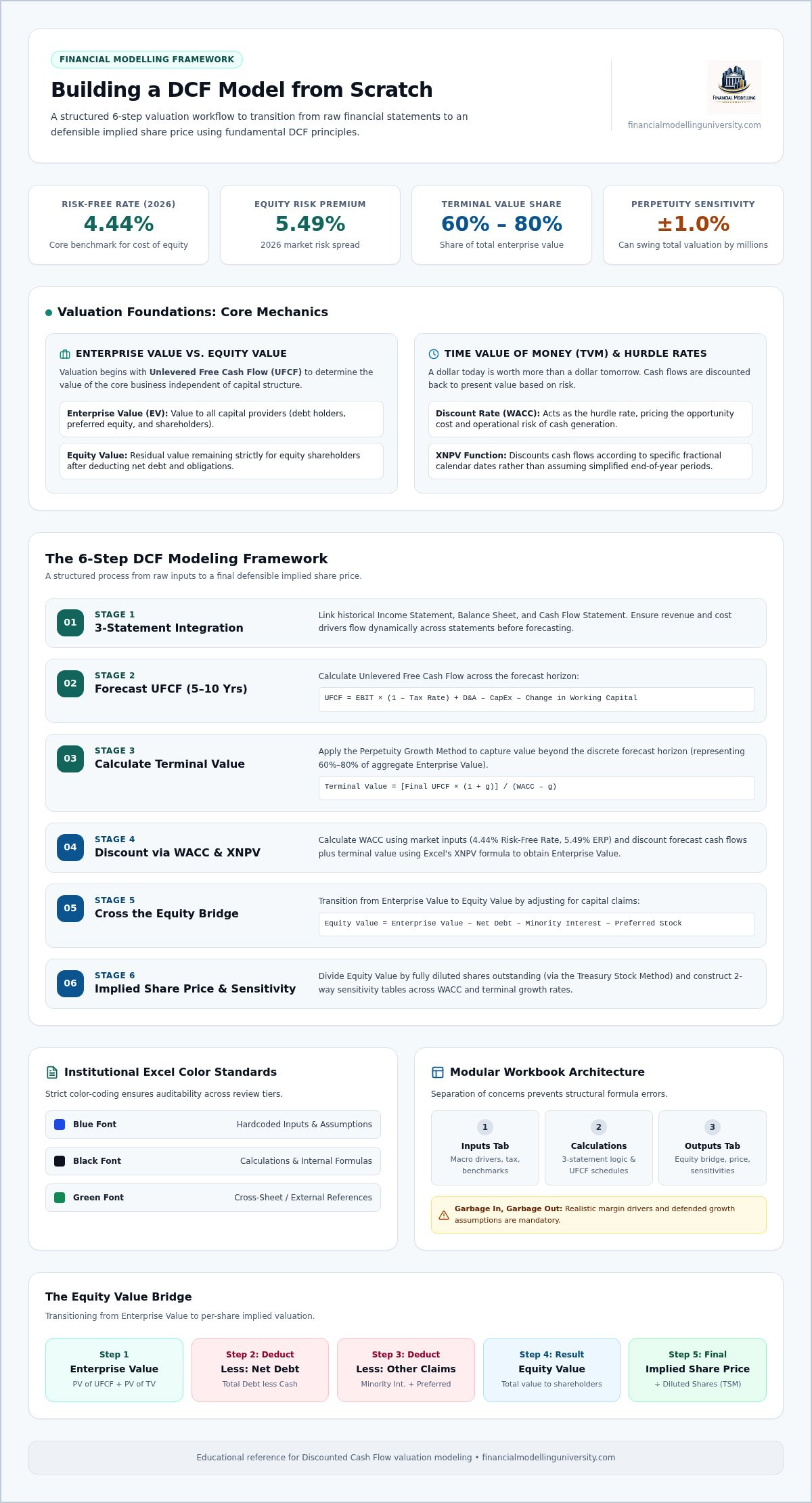
We’ll show you how to apply current 2026 market data, including the 4.44% risk-free rate and the 5.49% equity risk premium, to create a valuation that commands respect. You’ll move through forecasting unlevered free cash flows, calculating a precise terminal value, and performing the final sensitivity analysis. By the end of this guide, you’ll possess the technical discipline required to secure and excel in a high-prestige finance role.

The Fundamentals of DCF Valuation: Why Intrinsic Value Still Rules

The Discounted cash flow (DCF) analysis is the bedrock of fundamental finance. It defines a company’s worth as the present value of every dollar it will ever generate, adjusted for the risk of those cash flows actually materializing. While other methods rely on market sentiment or peer multiples, the DCF looks inward. It asks a simple, brutal question: what is the cash worth? Learning how to build a dcf model from scratch is about moving beyond superficial metrics to find a company’s true intrinsic value.

To model like a pro, you must distinguish between Enterprise Value and Equity Value from the first cell. Enterprise Value represents the total value of the business to all capital providers, including debt holders and preferred stockholders. Equity Value is what remains for shareholders after all debt is settled. Professional models focus on Unlevered Free Cash Flow (UFCF) to derive Enterprise Value first. This ensures the capital structure doesn’t distort your view of the underlying business performance.

The DCF remains the gold standard for valuation because it forces you to defend your assumptions. However, the “garbage in, garbage out” rule is absolute. If your revenue growth projections are unrealistic or your margin assumptions are flawed, the final output is worthless. A 1% change in your terminal growth rate can swing a valuation by millions. Precision is the baseline, but disciplined judgment is what separates an elite analyst from a data entry clerk.

Intrinsic Value vs. Market Price

In 2026, market volatility remains a constant. Speculative trends and algorithmic trading frequently disconnect stock prices from economic reality. Fundamental analysis allows you to ignore this noise. By focusing on cash flow, you identify if an asset is truly undervalued or if it’s merely riding a temporary wave of hype. Institutional-grade models provide the “why” behind an investment thesis. This gives you the confidence to hold a position when the market panics or sell when it becomes irrationally exuberant.

The Concept of Time Value of Money (TVM)

A dollar today is worth more than a dollar tomorrow. Inflation and opportunity cost dictate this reality. In your model, the discount rate acts as the hurdle rate. It accounts for the risk that future cash flows might not arrive as planned. The Present Value formula is your engine. It mathematically pulls future earnings back to today’s terms. Without mastering TVM, you’re just guessing. With it, you’re calculating the exact price an investor should pay for future growth.

The 6-Step Framework: Building the DCF Model in Excel

A professional model isn’t a single sheet of chaos. It’s a structured engine. Understanding how to build a dcf model from scratch requires a modular approach. Separate your work into clear tabs: Inputs, Calculations, and Outputs. This structure is standard in investment banking. Use color-coding religiously. Hardcoded numbers must be blue. Formulas must be black. References to other sheets should be green. This isn’t just about aesthetics; it’s about auditability.

Step 1 & 2: Forecasting Unlevered Free Cash Flow (UFCF)

Forecasting is where the real work happens. It’s the most time-intensive part of learning how to build a dcf model from scratch. You aren’t just projecting numbers; you’re projecting a business narrative. We use Unlevered Free Cash Flow (UFCF) because it represents the cash available to all capital providers, stripping away the noise of interest expense. The formula is: EBIT * (1 – Tax Rate) + Depreciation & Amortization – Capital Expenditures – Change in Net Working Capital. Note that the 2026 US Federal Corporate Tax Rate remains 21%. Net Working Capital is the most overlooked driver in junior models because it directly captures the cash trapped in day-to-day operations.

Step 3 & 4: Calculating Terminal Value and Discounting

Once you have your forecast period, usually five to ten years, you must account for the business’s value beyond that window. This is the Terminal Value. It often accounts for 60% to 80% of the total valuation. To discount these cash flows back to the present, use the XNPV function in Excel. Standard NPV assumes annual periods, but XNPV allows for specific dates, providing the precision required for institutional-grade work. For a deeper dive into the theory, Harvard Business School’s guide to DCF provides excellent academic context for these discounting mechanics.

Step 5 & 6: From Enterprise Value to Implied Share Price

The transition from Enterprise Value to an implied share price requires crossing the “Equity Bridge.” Subtract Net Debt, Minority Interest, and Preferred Stock to find the Equity Value. To get the final output, divide this by the fully diluted shares outstanding. Use the Treasury Stock Method to account for in-the-money options and warrants. If your final implied price is significantly different from the current trading price, re-examine your assumptions. Mastering this transition is a core component of our Investment Banking Financial Modeling Course, where we build these bridges from a blank sheet.

Terminal Value and Institutional-Grade Adjustments

The terminal value is the heaviest component of your valuation engine. In most professional models, this single calculation accounts for 60% to 80% of the total enterprise value. Because it carries such immense weight, a minor error in your terminal assumptions will invalidate the entire project. When learning how to build a dcf model from scratch, you must decide between two primary methodologies: the Perpetuity Growth Method and the Exit Multiple Method. Each has a specific application depending on the industry and the investment thesis.

Perpetuity Growth vs. Exit Multiple Method

The Perpetuity Growth Method, or Gordon Growth Model (GGM), assumes the business will grow at a constant rate forever. This is best suited for mature, stable companies in “old economy” sectors. Conversely, the Exit Multiple Method applies a valuation multiple (like EV/EBITDA) to the final year’s financial metric. This is the preferred approach in Private Equity and M&A because it reflects how the market actually prices businesses at the point of sale.

Avoid the “rookie” mistake of setting a perpetuity growth rate higher than the long-term GDP growth rate. If a company grows faster than the global economy indefinitely, it eventually becomes the global economy. Most elite analysts cap this rate between 2% and 3% to remain defensible during an associate review.

Advanced Adjustments: The Mid-Year Convention

Standard Excel models often assume all cash flows arrive on December 31. In reality, a business generates cash every day. Discounting from the end of the year systematically understates the value of the business because it ignores the time value of the money earned in January through November. To fix this, institutional models use the mid-year convention. You adjust your discount periods to 0.5, 1.5, and 2.5 instead of whole integers. This simple shift pulls cash flows forward by six months on average. The mid-year convention is a mandatory requirement for any model intended for an investment committee or high-stakes valuation. Mastering these nuances is what transforms a basic tutorial into a professional-grade work product. If you’re serious about how to build a dcf model from scratch at an elite level, these adjustments are non-negotiable.

Calculating WACC and Executing Sensitivity Analysis

The Weighted Average Cost of Capital (WACC) is the hurdle rate that defines your entire valuation. It represents the opportunity cost for every capital provider involved, both debt holders and equity investors. When you master how to build a dcf model from scratch, you realize that WACC isn’t just a static number; it’s a reflection of the market’s perception of risk. To maintain institutional-grade accuracy, you must always use the market value of debt and equity. Book values are historical artifacts. They have no place in a forward-looking valuation engine.

To calculate the Cost of Equity, elite analysts rely on the Capital Asset Pricing Model (CAPM). As of July 2026, the risk-free rate sits at 4.44%, based on the 10-Year Treasury yield. Combined with a current equity risk premium of 5.49%, your formula becomes: Cost of Equity = 4.44% + (Beta * 5.49%). This precision is what senior associates expect during a model audit. If your discount rate is off by even 50 basis points, your final Enterprise Value will be fundamentally flawed.

The Mechanics of WACC

Calculating a defensible Beta requires looking beyond a single company. You must identify a “Peer Group” of comparable public companies to derive an industry-standard risk profile. The process involves unlevering the Beta of each peer to strip away the effects of their specific capital structures. You then re-lever the average industry Beta using your target company’s specific debt-to-equity ratio. This ensures your WACC accurately reflects the business risk of the industry and the financial risk of the company’s leverage. Additionally, your Cost of Debt must be tax-effected. Using the 21% US Federal Corporate Tax Rate, the formula is: Rd * (1 – 0.21). This reflects the interest tax shield, a critical driver of value in any leveraged environment.

Sensitivity Tables and the ‘Football Field’ Chart

A single “target price” is a red flag in professional finance. It suggests a lack of understanding regarding market volatility. Institutional models use 2D Data Tables to show a range of possible outcomes. By sensitizing WACC against your Terminal Growth Rate, you create a matrix of values that accounts for different economic scenarios. This allows you to present a “valuation range” rather than a solitary, fragile number.

To finalize your presentation, summarize these findings in a “Football Field” chart. This visualization compares your DCF results against other methodologies, such as Trading Comps and Precedent Transactions. It provides the context necessary for a Managing Director to make an informed decision. If you want to master these advanced presentation techniques, our DCF Valuation Course provides the step-by-step blueprints used by top-tier firms. Understanding how to build a dcf model from scratch is the first step, but executing rigorous sensitivity analysis is what proves your professional “judgment.”

Mastering Valuation: From Tutorial to Industry Professional

Building your first model is a rite of passage. It marks your transition from a student of finance to a serious practitioner. Learning how to build a dcf model from scratch isn’t just an exercise in Excel; it’s a test of your ability to synthesize a company’s entire economic future into a single, cohesive narrative. While technical proficiency is the baseline, your ability to defend your “judgment” is what will set you apart in a high-stakes interview or a boardroom. Elite firms don’t just hire people who can use a calculator; they hire professionals who can think critically about risk and reward.

Common DCF Mistakes to Avoid in Interviews

Common mistakes often derail promising candidates during technical rounds. Avoid mismatching your cash flows and discount rates. Never discount Levered Free Cash Flow at WACC; it’s a fundamental error that signals a lack of core understanding. Similarly, aggressive long-term growth rates that exceed GDP projections will be shredded by any senior associate. You must also ensure your model’s structural integrity by mastering Excel for Finance fundamentals. A messy workbook suggests a messy mind. If your logic isn’t transparent, your valuation isn’t credible. Most interviewers look at your formatting before they even check your enterprise value.

Accelerate Your Career with FMU

FMU exists to bridge the gap between academic theory and the brutal reality of Wall Street. Our DCF Valuation Course is designed to transform you into an industry expert. You’ll move beyond simple tutorials to build complex, institutional-grade models from a blank sheet. We teach you to navigate the nuances of 2026 market data with the same confidence as a seasoned associate. You will learn to handle the complexities of circular references, tax shields, and mid-year conventions without breaking your model’s logic.

In a job market where technical skills are non-negotiable, a globally recognized certification from FMU serves as quantitative proof of your expertise. It’s a signal to employers that you possess the discipline required for high-stakes modeling. Mastering how to build a dcf model from scratch is the definitive entry ticket to elite tiers of investment banking and private equity. Choose the path of professional mastery. Secure your seat in the next cohort and start performing at the level of the industry’s top practitioners.

Master the Art of Institutional Valuation

Mastering the DCF is the ultimate differentiator in high-stakes finance. You now understand how to build a dcf model from scratch by integrating 3-statement logic, calculating a defensible WACC using current 2026 benchmarks, and applying institutional adjustments like the mid-year convention. These technical hurdles are no longer barriers to your advancement. They are the tools you will use to justify multi-billion dollar investment theses.

Transitioning from basic tutorials to professional execution requires a proven blueprint. Our curriculum is designed by former bulge-bracket investment bankers to ensure you perform at the highest level. Trusted by 25,000+ finance professionals, FMU provides the institutional-grade Excel templates and rigorous training necessary for complete career transformation. Don’t settle for entry-level skills when you can command the room with expert-level precision.

Enroll in the FMU DCF Valuation Course and Master Professional Modeling

Take command of your professional trajectory today. The path to mastery is disciplined and highly structured. We’re ready to guide you to the top of the industry.

Frequently Asked Questions

What is the difference between Unlevered and Levered Free Cash Flow in a DCF?

Unlevered Free Cash Flow (UFCF) represents the cash available to all capital providers, including both debt holders and equity investors. It’s calculated before interest payments and is used to derive Enterprise Value. Levered Free Cash Flow (LFCF) is the cash remaining for shareholders after all debt obligations are met. Most institutional analysts prefer UFCF because it allows for a cleaner comparison of operating performance regardless of a company’s specific capital structure.

How many years should my DCF forecast period be?

A standard forecast period typically spans five to ten years. The objective is to project cash flows until the company reaches a “steady state” where its growth and margins are predictable. For mature companies, a five-year forecast is usually sufficient. High-growth firms or those in cyclical industries often require a ten-year window to capture the full transition to long-term stability.

Is the DCF model still used in Private Equity and M&A?

The DCF remains a fundamental pillar of valuation in both Private Equity and M&A. While Private Equity firms rely heavily on LBO models to determine returns, they use the DCF as a critical sanity check for intrinsic value. In M&A, it helps buyers determine the maximum price they can pay while still achieving their required internal rate of return. It provides the “floor” valuation that multi-billion dollar deals are built upon.

How do I choose the right Terminal Growth Rate?

Select a Terminal Growth Rate that aligns with the long-term inflation rate and the expected growth of the broader economy. Institutional models typically cap this rate between 2% and 3%. You must never set this rate higher than the GDP growth rate. If a company grows faster than the economy forever, it would eventually become larger than the entire market, which is a logical impossibility that senior associates will immediately flag.

What happens if my WACC is higher than my growth rate?

Your WACC must be higher than your terminal growth rate for the Gordon Growth formula to function correctly. If the growth rate exceeds the discount rate, the denominator becomes negative, leading to an infinite or nonsensical valuation. This mathematical reality is a core reason why learning how to build a dcf model from scratch requires such disciplined assumptions. Real-world companies cannot sustain hyper-growth indefinitely without eventually hitting the ceiling of the discount rate.

Can I build a DCF model for a company with negative EBITDA?

You can model a company with negative EBITDA as long as you can defensibly project a path to profitability within the forecast period. The DCF is forward-looking; it values future cash, not current losses. You must clearly identify the specific “inflection point” where operating leverage kicks in and margins turn positive. If the company never generates positive cash flow in your model, its intrinsic value is zero.

What is the Treasury Stock Method and why does it matter for DCF?

The Treasury Stock Method (TSM) is used to calculate a company’s fully diluted shares outstanding by accounting for “in-the-money” options and warrants. It assumes that any proceeds from the exercise of these options are used by the company to repurchase shares at the current market price. This is vital for moving from Enterprise Value to Equity Value. Without TSM, you risk overstating the share price by ignoring the dilutive impact of employee compensation and warrants.

How often should a DCF model be updated?

Update your DCF model quarterly or after any major market event that shifts your core assumptions. Market-driven inputs, such as the 4.44% risk-free rate or the 5.49% equity risk premium, are dynamic and impact your WACC immediately. When you understand how to build a dcf model from scratch, you’ll see that even a small shift in the cost of capital can significantly alter your target price. Professional models are living documents, not static spreadsheets.